Microphone-Results-Analysis-1
Results
I’ve built quite a few microphone circuits in the last few months since I have updated this project, and in the process I learned a tremendous amount– in addition to everything about the microphones, pre-amps etc., but also about circuit board layout and manufacture. Until now, I’ve had very limited experience fabricating PCBs (I imagine because I never considered it an option due to my own lack of skill), but since committing to learning it seems there to be an endless list of boards I want to work on. Some things I learned off the bat:
- Silk-screens are not optional – well, I suppose they are, but it sure helps if you put the time in ensuring parts are labeled well, and terminals have the polarity written on them (if I can plug it in backwards, I probably will unless it is written on the board).
- Reverse voltage, over-voltage, over-current protection are also worth designing into the board. It saves time and cost in the long-run.
- Test points are much easier to probe than little pads of SMD components.
- Adding features such as room for jumpers, 0 Ohm resistors etc. is very easy in CAD, and barely takes room on the board, and they don’t need to be populated if they aren’t used.
- I recall in EOD there was a saying “neat demo is good demo”, well a neat PCB is a good PCB. At least for me, every time I tidy up the circuit I catch mistakes.
- Auto-router is not worth using (I’m sure it has a role, but not for the majority of the routing). I like routing the boards. First, doing it myself ensures the layout of components makes sense, and also it ensures the important traces (signals, power, etc.) are routed logically. It’s rather cathartic too.
That is obviously a non-exhaustive list, but before I get too side-tracked, I want to get back to the current results of the project at hand. Below is an audio clip recorded with my microphone, which is plugged into a cheap USB sound-card.
Now here is a “Blue Snowball” conenser microphone. It is ~$50 and gets very positive reviews for the most part.
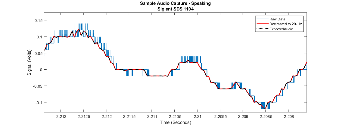
I also played with using my oscilloscope to record the audio (USB from the scope to my computer and saving the data in the EasyScope application). When I record this way it sounds terrible. The scope I was using only has an 8-bit ADC (analog to digital converter), so when you look at the waveforms it is immediately apparent that there is a digitizing issue.
Here is the waveform both raw and decimated to 20kHz.
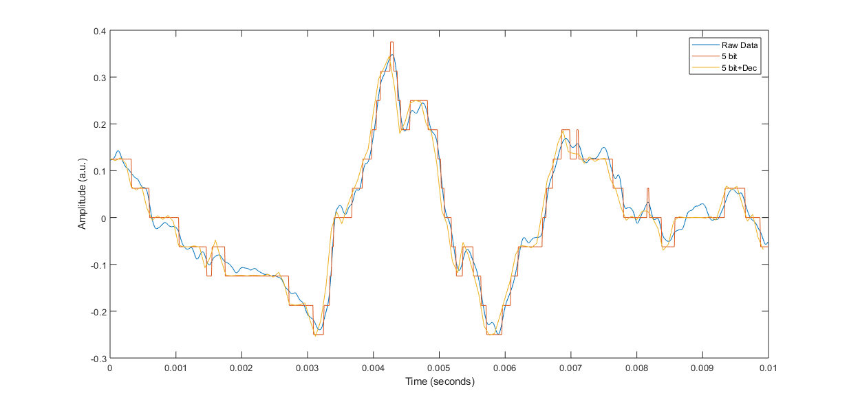
This bring up an interesting point, about sampling rate (I’ll get to hardware eventually, I promise). The scope can sample at hundreds of MHz, but there is only 8 bits of accuracy, and for audio purposes, ideally you would like up to 16 bits and 50kHz is plenty fast for sampling (Nyquist requires 34kHz if you can only hear up to 17kHz or so, and most audio is closer to 1-4kHz). To first demonstrate this in a bit of an extreme case, here are four audio clips: Raw audio from my microphone, that same audio digitized to 8-bits,6-bits,and 5-bits. Script (here)[/assets/Audio/Microphone/InitialTesting/Digitizing_Decimating]
While 5-bits sounds horrible, if you add a decimate it by a factor of 8 (according to MATLAB’s documentation, “By default, decimate uses a lowpass Chebyshev Type I infinite impulse response (IIR) filter of order 8”) Basically, it reduces the sampling rate by a factor N (8 here) and smooths out the data some. It is not a rolling average, though. Here is just the decimated sound:
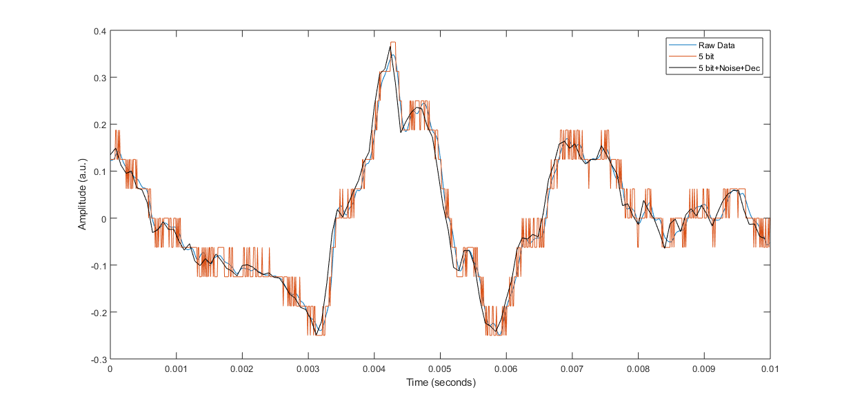
But decimation has a challenge– if the data is too quiet (i.e. there isn’t enough noise), then it just has digital flats as the original did. But if the data is a little noisy and jumps around, the decimation can work properly. And to be clear, the noise needs to be added before the digitization, not after. If the noise is after the digitization the decimation will just smooth out that noise and not work properly. Below is a sound clip that has noise added to the raw data roughly to the level of 1 least significant bit (2^-4) for 5 bit.
Here are the plots of the waveforms in the different cases. First is the raw data, 5 bit data, and then the 5 bits decimated by a factor of 8. The second plot has the raw data, then the 5 bit version of the raw data (with noise added), and finally a decimated waveform. Notice how without noise the 5 bit data has lots of flat regions? And the decimated wave matches those flats, but in the noisy version there is a pulse-width modulation effect going on due to the noise. So even though it has some extra noise, it actually helps.